Using CUDA to generate Julia sets
I was curious to see if I could find a more relevant example of how CUDA speeds up calculations. One example where it helps is with calculating Julia sets. Julia sets are sets that are found by iterating a mapping z → z*2+c for some complex number c and seeing which points escape. For a detailed description, see the Wikipedia page https://en.wikipedia.org/wiki/Julia_set.
The reason I like the example with Julia sets is that these are calculated pixel-per-pixel, i.e., we check for each point independently if it falls within the Julia set. This means it’s we have a lot of similar calculations that can happen in parallel. The calculations are also relatively simple. So, from the last post we know this means CUDA will perform relatively well here.
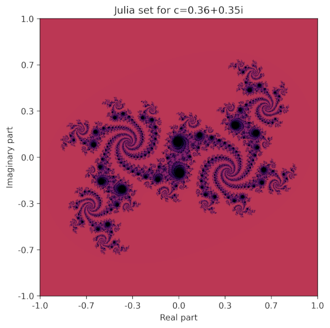
I set the parameters as follows. We calculate the Julia set for a 1000 by 1000 grid and we perform 1000 iterations to see if points escape. We will record how many iterations it takes for a point to escape and color the plot based on this number of iterations.
# Parameters
n = 1000 # Number of points per axis.
iterations = 1000 #Iterations to run the Julia set algorithm.
c = 0.36+0.35*1j # c in the equation z^2+c
scale = 1.35 # Zoom in and out of the set.
We need some libraries:
import numpy as np
import cupy
import itertools
import matplotlib.pyplot as plt
import time
from math import sqrt
The NumPy code is as follows:
# NumPy calculation
np_start = time.time()

julia_array = np.empty([n+1, n+1],dtype=complex)
iteration_array = np.zeros([n+1, n+1],dtype=float)

x_coords, y_coords = np.meshgrid(np.arange(n+1), np.arange(n+1), indexing='ij')
julia_array = scale*(1-(2*x_coords/n)) + scale*((2*y_coords/n)-1)*1j

R = (1+sqrt(1+4*abs(c)))/2 # Quadratic equation to find escape radius

for _ in range(iterations):
    julia_array = julia_array*julia_array+c
    julia_array = np.where(np.abs(julia_array) > R, R, julia_array)
    escaped = np.abs(julia_array) == R # Points that have escaped the set.
    iteration_array = np.where(escaped, iteration_array, iteration_array+1)

iteration_array = iteration_array/iterations

np_time = time.time()-np_start
print(f"NumPy runtime {np_time:.3f}")
The CuPy code is as follows:
cupy_start = time.time()

julia_array = cupy.empty([n+1,n+1],dtype=complex)
iteration_array = cupy.zeros([n+1,n+1],dtype=float)

x_coords, y_coords = cupy.meshgrid(cupy.arange(n+1), cupy.arange(n+1), indexing='ij')
julia_array = scale*(1-(2*x_coords/n)) + scale*((2*y_coords/n)-1)*1j

R = (1+sqrt(1+4*abs(c)))/2 # Quadratic equation

for _ in range(iterations):
    julia_array = julia_array*julia_array+c
    julia_array = cupy.where(cupy.abs(julia_array) > R, R, julia_array)
    escaped = cupy.abs(julia_array) == R # Points that have escaped the set.
    iteration_array = cupy.where(escaped, iteration_array, iteration_array+1)

iteration_array = iteration_array/iterations

cupy_time = time.time()-cupy_start

print(f"CuPY runtime {cupy_time:.3f}")
On my PC the CuPy runtime is 0.861 seconds, while the NumPy runtime is 41.614 seconds. So, similar to the last post, using CuPy is roughly speeds up the code roughly 50 times.
Plotting the above code gives:
It can be generated with the following code:
#Code to plot the Julia set
plt.figure(figsize=(6, 6))
im = plt.imshow(-iteration_array, cmap='inferno', vmin=-1, vmax=1, origin='lower')
tick_positions = np.linspace(0, n, 7)
tick_labels = np.linspace(-1, 1, 7)
plt.xticks(tick_positions, [f'{x:.1f}' for x in tick_labels])
plt.yticks(tick_positions, [f'{x:.1f}' for x in tick_labels])

# Set title and labels
plt.title("Julia set for c=0.36+0.35i")
plt.xlabel('Real part')
plt.ylabel('Imaginary part')
plt.savefig("julia_set.png", dpi=300, bbox_inches='tight')